The Logistic Regression is an important classification model to understand in all its complexity. There are a few reasons to consider it:
- It is faster to train than some other classification algorithms like Support Vector Machines and Random Forests.
- Since it is a parametric model one can infer causal relationships between the response and explanatory variables.
- Since it can be viewed as a single layer neural network, it is useful to understand it to gain a deeper understanding of Neural Networks.
This article seeks to clearly explain the Binomial Logistic Regression, the model used in a binary classification setting.
The Logistic Regression has been around for a long, long time and while it is not going to single-handedly win any kaggle competitions, it is still widely used in the analytics industry. So, what can be a useful point of departure to understand the Logistic Regression intuitively? I actually like to begin with the Naive Bayes model and assume a binary classification setting. In Naive Bayes, we are trying to compute the posterior probability, or in simple terms, the probability of observing that our response variable (Y) is categorized as 1, given some specific values for our variables. The solution to the problem is expressed as:
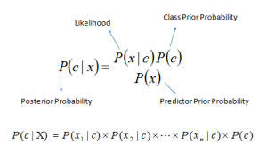
The goal of the Binomial Logistic Regression (Logistic Regression or LR for the remainder of this article) is exactly the same, to compute the posterior probability. However, in LR we will compute this probability directly.
The response variables (Y) follows a Binomial distribution (a special case of the Bernoulli distribution) and the probability of observing a certain value of Y (0 or 1) is:
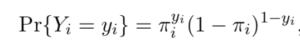
Note that if yi =1 we obtain πi ,and if yi =0 we obtain 1−πi. Now, we would like to have the probabilities πi depend on a vector of observed covariates xi. The simplest idea would be to let πi be a linear function of the covariates, say πi = x′iβ.
One problem with this model is that the probability πi on the left-hand- side has to be between zero and one, but the linear predictor x′iβ on the right-hand-side can take any real value, so there is no guarantee that the predicted values will be in the correct range unless complex restrictions are imposed on the coefficients.
A simple solution to this problem is to transform the probability to remove the range restrictions and model the transformation as a linear function of the covariates. Essentially what we are saying is that we want to map the output of our covariates (not necessarily including the intercept) to a continuous range which corresponds to {0-1}. We use the odds ratio to do this.
The odds ratio gives the probability of an event occurring (πi) over
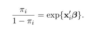
At this point it is useful to express πi , the probability of Y as a conditional probability of P(Y|X). If we were to solve for P(Y|X) we would arrive at the following expression:
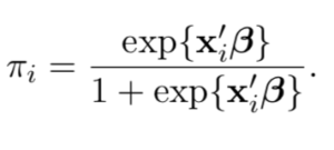
Now our posterior probability has been mapped to our covariates and the form of this function is called the sigmoid curve. Here is a visual representation.
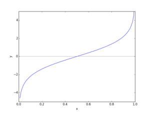
As you can see, the outputs are constrained between the range (0,1).
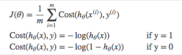
Now, what we seek to do is maximize the predicted probabilities as expressed above. Specifically, we will want to maximize P(Y=0|X) when we actually observe Y=0 AND maximize P(Y=1|X) when we observe a 1. Let us call this our objective function L(β). If we were to take the negative log of this expression we would arrive at
If we were to plot the two Cost equations above we would see:
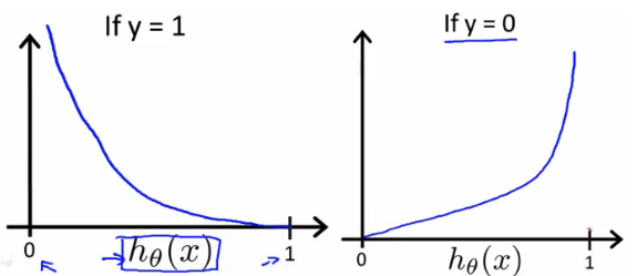
Since we have taken the negative log likelihood, we are now minimizing our loss function as opposed to maximizing it.
To fit (find the optimum coefficients) for our model we would take the derivative of the loss function with respect to β we would arrive at:
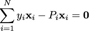
The term P here is our predicted probability P(Y|X).
Unfortunately, our loss function does not have a closed-form solution and we must arrive at our minimum via stochastic gradient descent. We already have the expression above that tells us now sensitive our Loss/error function is to a small change in β. So now we can plug that expression into the standard gradient update rule.

Voila! Now we have everything we want. Let's put it all together in Python now.
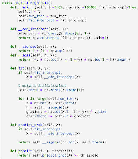
Love Data Science? Checkout our intro and immersive programs.